Opening Range Breakout: Real Edge or Backtest Illusion?
A futures-based evaluation with margin modeling and out-of-sample validation.

The Opening Range Breakout (ORB) is one of the most discussed intraday strategies in retail trading.
It has been tested, modified, optimized, and re-packaged countless times.
The goal here is not to present a “new” version of ORB, but to evaluate it under realistic conditions:
on a futures contract (MNQ),
with proper contract rollover handling,
using a back-adjusted continuous series,
with fixed commissions,
and explicit capital and margin modeling.
The entire process is documented in a reproducible research notebook, including:
the prepared dataset,
the engineering required to adapt backtesting.py to futures,
in-sample optimization,
and out-of-sample validation.
This is not the usual story on ORB.
Strategy Description
The strategy is trend-following and breakout-based.
It uses the opening range of the U.S. market. Although the reference asset is a futures contract (which trades almost continuously), it is ultimately driven by the underlying index components. The first minutes of regular trading are typically the most important in defining a price range — this is the so-called opening range.
The core hypothesis is simple:
If this range is broken to the upside, continuation to the upside becomes more likely.
If broken to the downside, continuation to the downside becomes more likely.
The strategy exits either via take profit, stop loss, or forcefully at the beginning of the next trading session (at an hour corresponding to the U.S. market open).
The illustration below shows a typical upside breakout above the opening range.
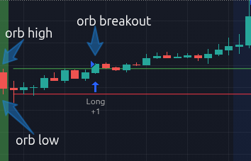
The only additional filter applied is a trend filter: a simple 200-day moving average.
If price is above the SMA(200), only long breakouts are considered.
If price is below, only short breakouts are considered.
ORB-type breakout systems tend to overtrade during sideways sessions, producing multiple small losses in the same day.
For this reason, I enforce a simple risk rule: stop trading after one losing trade in the same session. This is not optimized; it’s a fixed execution constraint.
Capital and Risk Management
The backtest assumes an initial capital of $10,000 and a position size of one MNQ contract (Micro Nasdaq).
Margin requirements for this setup typically fluctuate between $2,000 and $2,500.
Commissions are modeled as a fixed $0.68 per side, approximately in line with a broker such as Interactive Brokers.
The strategy uses a dynamic stop loss based on the opening range.
Once the upper and lower ORB levels are defined, if a trade is opened, the opposite side of the range becomes the stop level.
The take profit is determined by applying a risk-reward multiplier to that stop distance.
Because the stop is dynamic, during periods of high volatility the distance to the opposite ORB level may become too wide, potentially generating losses exceeding 2–3% of capital. This is not acceptable within this framework.
For this reason, a secondary static stop cap (in ticks) is applied.
Beyond this maximum threshold, the loss cannot increase further.
This ensures that risk remains bounded and measurable.
Data
The dataset provided with the notebook is ready to run.
The data begins in 2019 and was downloaded in raw format from Databento.
From this dataset, two dataframes were created: one in-sample and one out-of-sample, specifically structured for this strategy.
Futures rollover is handled by switching to the next contract approximately five trading days before expiration (or earlier if the next contract becomes more liquid, based on volume).
This avoids discontinuities caused by holding the expiring contract during the rollover window.
In practical terms, since the strategy remains in the market at most for one session and exits forcefully at the beginning of the next session, it is structurally impossible for a trade to span a contract switch.
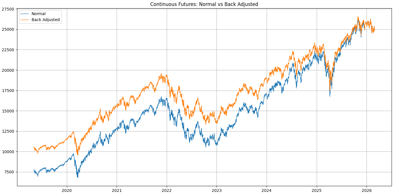
Additionally, a back-adjusted continuous series is used because the trend filter relies on a daily SMA(200), which requires a continuous price history without rollover gaps. Since trades never span rollover events, adjusted and non-adjusted series produce identical trade-level results.
Tools and Backtest Engineering
The backtest was conducted using the framework backtesting.py (URL).
The entire process is documented and fully reproducible through a notebook available to subscribers.
Since backtesting.py does not natively support futures contracts, several workarounds were required in order to accurately model the situation while preserving precise metrics and price calculations.
The first issue concerns capital ($10,000) versus the underlying price, which is higher than the available capital.
A leverage of approximately 20x was assumed, reflecting margin requirements that typically range between $2,000 and $2,500.
A lower leverage would also have worked, but the objective was to remain aligned with the idea that not all capital is deployed, and that risk per trade remains limited to a small percentage of capital.The second issue concerns position sizing.
I want to trade one contract. However, one MNQ contract moves $2 per index point (0.25 tick size, $0.50 per tick).
Profit and loss are determined by the point difference between entry and exit.Since backtesting.py does not reason in “points” but in price differences, the simplest solution is to use a position size of 2.
For example:
If price moves from 24,950 to 25,000, that is 50 index points, corresponding to $100 in PnL for one MNQ contract.
The raw price change is 50, so by using size=2 the monetary calculation aligns correctly.Commissions remain fixed per side, so no further adjustment is required.
Full Optimization Results & Research Notebook
The complete research notebook includes:
Full optimization runs
Heatmaps
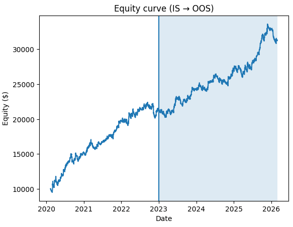
In-sample / Out-of-sample split
Equity curve stitching
Trade log verification
All engineering workarounds
Subscribers can access the full notebook and dataset below.
Optimization
Parameter optimization was performed on the in-sample dataset using the built-in optimizer of backtesting.py.
The objective function was the Sharpe Ratio, which allows comparison of configurations based on risk-adjusted returns rather than raw profitability.
The maximum stop distance was fixed at 150 ticks, corresponding to a maximum loss of approximately $75 per trade (less than 1% of the initial $10,000 capital).
This cap is applied purely as a risk constraint, preventing excessively large losses during highly volatile sessions when the ORB range becomes unusually wide.
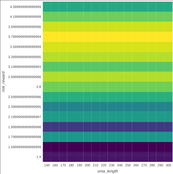
This is the optimization grid used:
mnq_optimization_grid = {
    "sma_length": range(150, 301, 10),
    "risk_reward": list(np.arange(1.4, 4.4, 0.2)),
}
By keeping the stop cap fixed, the optimization is restricted strictly to strategy parameters, avoiding the common pitfall of tuning risk limits directly on historical data.
The optimization grid was therefore limited to two parameters:
sma_length — the lookback period of the trend filter
risk_reward — the take-profit multiple relative to the ORB stop distance
The objective of the optimization is not to find a single “perfect” parameter combination, but rather to evaluate whether a stable region of profitability exists within a reasonable parameter space.
Strategies whose performance exists only at a single precise parameter coordinate are often the result of curve fitting, whereas strategies that perform well across a broad region of parameter values are more likely to reflect a genuine structural edge.
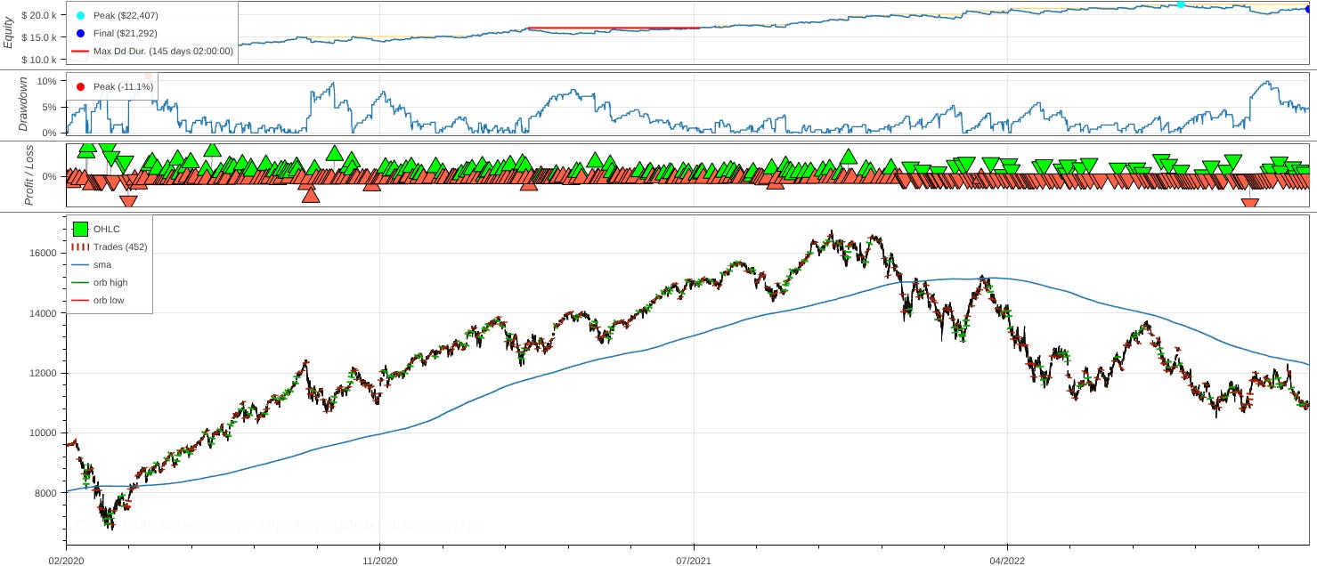
In Sample
In-sample results are solid. The win rate is not high, which is typical for breakout systems, but risk-adjusted performance remains strong.
Performing another type of optimization for example using “Win Rate [%]” metric, the Win Rate arise above 40% but sharpe decrease.
Start                     2020-02-12 08:30...
End                       2022-12-30 15:00...
Duration                   1052 days 06:30:00
Exposure Time [%]                    25.77845
Equity Final [$]                     20863.94
Equity Peak [$]                      22034.76
Commissions [$]                        613.36
Return [%]                           108.6394
Buy & Hold Return [%]                15.36432
Return (Ann.) [%]                    27.94332
Volatility (Ann.) [%]                20.33923
CAGR [%]                              19.2586
Sharpe Ratio                          1.37386
Sortino Ratio                         3.46301
Calmar Ratio                          2.56241
Alpha [%]                           107.96951
Max. Drawdown [%]                   -10.90507
Avg. Drawdown [%]                     -0.9807
# Trades                                  451
Win Rate [%]                         30.37694
Profit Factor                          1.4291
The heatmap does not show a single isolated optimum. Instead, performance is distributed across a relatively smooth region of the parameter space. This reduces the probability that the observed edge is the result of parameter overfitting.
Out of Sample
Start                     2023-01-03 08:30...
End                       2026-02-27 15:00...
Duration                   1151 days 06:30:00
Exposure Time [%]                     24.0189
Equity Final [$]                     19457.86
Equity Peak [$]                      21844.76
Commissions [$]                        644.64
Return [%]                            94.5786
Buy & Hold Return [%]               127.58833
Return (Ann.) [%]                    23.17691
Volatility (Ann.) [%]                21.02388
CAGR [%]                             15.68568
Sharpe Ratio                          1.10241
Sortino Ratio                         2.70307
Calmar Ratio                          1.81298
Alpha [%]                            64.60328
Max. Drawdown [%]                   -12.78384
Avg. Drawdown [%]                    -1.27488
# Trades                                  474
Win Rate [%]                         24.89451
Profit Factor                         1.32135
Interpretation of Results
In-sample, the strategy outperforms buy & hold.
Out-of-sample, it does not consistently outperform in absolute terms.
However, this comparison alone is incomplete.
The maximum drawdown is significantly lower than the underlying index.
This is reflected in a Sharpe ratio close to 1 in out-of-sample testing.
More importantly, the strategy spends a limited amount of time in the market.
Capital is frequently idle and therefore available for allocation to other strategies.
The objective was not to outperform buy & hold in absolute terms,
but to evaluate whether the ORB structure exhibits a persistent, measurable edge under realistic assumptions.
The out-of-sample results suggest that while performance naturally degrades compared to in-sample, the structural edge remains present.
ORB is not a magical strategy.
But when engineered and tested properly, it does not appear to be a backtest illusion either.